Stochastic Taylor Derivative Estimator (STDE)
Jan. 13, 2025How to tackle the curses of dimensionality and the exponential curse in derivative order.
\(\require{physics}\newcommand{\I}{\text{i}}\DeclareMathOperator*{\argmax}{arg\,max}\DeclareMathOperator*{\argmin}{arg\,min}\)
The problem
Suppose we want to solve optimization problems where the loss function \(f\) contains differential operators
\begin{equation*} \label{eq:opt-diff} \argmin_{\theta} f(\mathbf{x}, u_{\theta }(\mathbf{x}), \mathcal{D}^{\alpha^{(1)} } u_{\theta }(\mathbf{x}), \dots, \mathcal{D}^{\alpha^{(n)} } u_{\theta }(\mathbf{x})), \quad u_{\theta }:\mathbb{R}^{d} \to \mathbb{R}^{d’}. \end{equation*}
where \(u_{\theta }\) is a neural network. A prominent example of this problem is physics-informed neural networks (PINN), where the loss is the PDE residual.
Naturally, we will be using auto-diff (AD) to handle the differential operators \(\mathcal{D}^{\alpha^{(i)} }\). But how to handle high-order derivatives like \(\pdv[2]{u_{\theta }}{x}\)? The simplest way would be to apply backward mode AD (backpropagation) twice. In JAX this can be done as
jax.grad(jax.grad(u))
and in PyTorch
u_x = torch.autograd.grad(u(x), x, create_graph=True)[0]
u_xx = torch.autograd.grad(u_x, x)[0]
However, doing this presents curses of dimensionality and exponential curse of order! After doing some asymptotic analysis, one would find that the memory scaling is \(\order{{\color{red}2^{k-1}}({\color{BurntOrange}d}+(L-1)h)}\), and the compute scaling is \(\order{{\color{red}2^{k}}({\color{BurntOrange}d}h+(L-1)h^{2})}\). Notice the curses of dimensionality and the exponential curse in derivative order.
Why applying backward mode AD repeatedly is bad
Now let’s look into the compute graph of repeated backward mode AD and see why it is a bad idea. Suppose we have a \(4\) layer MLP \(u=F_{4}\circ F_{3} \circ F_2 \circ F_1\) with hidden size \(h\). Denotes the activation as \(\vb{y}_{i}=F_{i}(\vb{y}_{i-1})\) and intermediate cotangents be \(\vb{v}_{i}^{\top}=\vb{v}_{i-1}^{\top}\pdv{F_{L-i+1}}{x}\).
Performing backward mode AD computes the vector-Jacobian-product (VJP) \(\vb{v}^{\top}\pdv{F}{\vb{x}}\) with the cotangent \(\vb{v}^{\top}=1\). The first row of the compute graph below depicts the VJP: first the forward pass is performed, then the backward pass is performed. Notice that the backward pass can only be performed once the forward pass is completed since the activations are needed.
Now suppose we apply VJP twice. This essentially treats the entire VJP compute graph (the blue box) as the forward pass, and as before a backward pass is created for each node in the forward pass, and we now have twice as many activations to store:
From this, we see that the compute graph doubles with every repeated application of backward mode AD, which is the origin of the exponential curse in derivative order.
Amortization
The cost of an expensive operation can be amortized over an iterative optimization procedure by using a cheap stochastic estimator. The most well-known example is the stochastic gradient descent (SGD), which uses estimated gradient that can be computed cheaply instead of the full gradient:
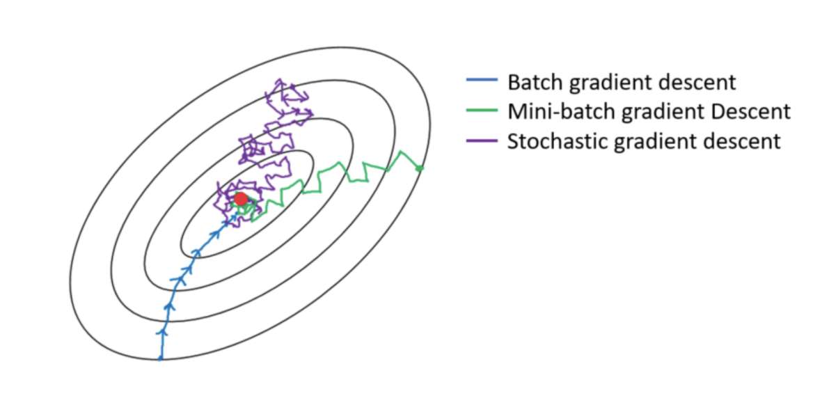
Figure 1: stochastic gradient descents
The idea of SGD was extended to differential operators in a recent work SDGD (Hu et al. 2023). Take the The Laplacian operator as an example. Laplacian of a function is the sum of diagonal elements of its Hessian. If we treat these diagonal elements as data, at each gradient descent step we can use a mini-batch of data instead of the full batch, by sampling uniformly among these diagonal elements:
\begin{equation} \laplacian =\sum_{i=1}^d \pdv[2]{}{x_{i}} \approx \frac{1}{B}\sum_{j}^B \pdv[2]{}{x_{I_{j}}} \end{equation}
Essentially SDGD converts a d-dim problem into \(B\) 1-dim problems. By employing amortization, SDGD effectively removes the curse of dimensionality:
- memory complexity: \(\order{{\color{red}2^{k-1}}({\color{orange}d}+(L-1)h)} \to \order{{\color{orange}B} ({\color{red}2^{k-1}}({\color{orange}1}+(L-1)h))}\).
- computation complexity: \(\order{{\color{red}2^{k}}({\color{orange}d}h+(L-1)h^{2})} \to \order{{\color{orange}B}{\color{red}2^{k}}(h+(L-1)h^{2})}\).
With SDGD, one can solve \(100,000\) dimensional PDEs with a 40GB A100 GPU in around 12 hours. Certainly a big step forward, but the exponential curse of derivative order persists if one looks at the asymptotics above. The amortization would be much more efficient if the exponential scaling in derivative order is reduced. This is exactly the goal of STDE (Shi et al. 2024).
Generalizing Hutchinson trace estimator (HTE)
The construction of STDE is very much inspired by HTE (Hutchinson 1989), which is a cheap stochastic estimator for matrix trace. The gist of HTE can be written down in just a few lines
\begin{equation} \begin{split} \tr(\vb{A}) =& \mathbb{E}_{\vb{v} \sim p(\vb{v})}\left[ \vb{v}^{\mathrm{T}} \vb{A} \vb{v}\right] =\vb{A} \cdot {\color{grey}\mathbb{E}_{\vb{v} \sim p(\vb{v})}\left[ \vb{v} \vb{v}^{\mathrm{T}}\right]} =\vb{A} \cdot {\color{grey}\vb{I}}, \quad \vb{v} \in \mathbb{R}^d \\ \approx& \frac{1}{B} \sum_{\vb{v}^{(i)}} \vb{v}^{\mathrm{T}} \vb{A} \vb{v}, \quad \vb{v}^{(i)} \sim p(\vb{v}) \end{split} \end{equation}
where the highlighted part, i.e. the distribution \(p\) is isotropic, is the constraint that must be satisfied for the equality to hold. Geometrically, this constraint can be understood as a random projection \(\vb{v} \vb{v}^{\mathrm{T}}\) that is a constant map in expectation.
HTE can be applied to provide a stochastic estimation of the Laplacian since the Laplacian is the trace of Hessian. Can we extend the construction for arbitrary differential operators? The first step is to write a differential operator \(\mathcal{L}\) in the following form:
\begin{equation} \mathcal{L}u(\vb{a}) =D^{k}_{u}(\vb{a}) \cdot \vb{C}(\mathcal{L}). \end{equation}
where \(D^{k}_{u}(\vb{a})\) is the kth order derivative tensor of \(u\) at point \(\vb{a}\), and \(\vb{C}(\mathcal{L})\) is a coefficient tensor of the same shape as \(D^{k}_{u}(\vb{a})\). For example, the Laplacian can be written in this form as
\begin{equation} \laplacian u(\vb{a}) = \sum_{i=1}^d \pdv[2]{u}{x_{i}} = D^{2}_{u}(\vb{a}) \cdot {\color{grey}\underbrace{\vb{I}}_{C(\laplacian)}}. \end{equation}
So HTE applied to the Laplacian can be interpreted as a randomized rank-1 decomposition of the coefficient tensor \(\vb{I}\). To generalize the idea for arbitrary differential operator, one just needs to replace the isotropic condition with a randomized rank-1 decomposition of a general coefficient tensors \(\vb{C}(\mathcal{L})\):
\begin{equation} \mathbb{E}_{p}\left[\otimes_{i=1}^{k}\vb{v}^{(v_i)}\right] = \vb{C}(\mathcal{L}) \end{equation}
With distribution \(p\) satisfying the above, we can write the action of the differential operator on the network \(u\) as an expectation over random projections of \(D^{k}_{u}\), which can be estimated via Monte Carlo:
\begin{equation} \mathcal{L}u(\vb{a}) = \mathbb{E}_{p}\left[D^{k}_{u}(\vb{a}) \cdot \otimes_{i=1}^{k}\vb{v}^{(v_i)}\right]. \end{equation}
The challenge now is to compute the random projection \(D^{k}_{u}(\vb{a}) \cdot \otimes_{i=1}^{k}\vb{v}^{(v_i)}\) efficiently. One would need to avoid computing the full derivative tensor \(D^{k}_{u}\) since it grows exponentially to the derivative order \(k\):
- \(k=1\) (Jacobian):
\begin{align*} D^{1}_{u}=\mqty[ \pdv{u}{x_{1}} & \dots & \pdv{u}{x_{d}}] \in \mathbb{R}^{d} \end{align*}
- \(k=2\) (Hessian):
\begin{align*} D^{2}_{u}=\mqty[ \pdv{u}{x_{1}}{x_{1}} & \dots & \pdv{u}{x_{1}}{x_{d}} \\ \vdots & & \vdots \\ \pdv{u}{x_{d}}{x_{1}} & \dots & \pdv{u}{x_{d}}{x_{d}} \\ ] \in \mathbb{R}^{d\times d} \end{align*}
- \(k=3\): \(D^{3}_{u}=\mqty[ \frac{\partial ^{3} u}{ \partial x_{i} \partial x_{j} \partial x_{k}} ]_{ijk} \in \mathbb{R}^{d\times d\times d}\)
It turns out that one can use high-order directional derivatives to compute the said random projection efficiently. In the following, we will discuss
- how to express arbitrary projection of the derivative tensor to high-order directional derivatives, and
- how high-order directional derivatives can be computed efficiently.
High-order directional derivatives
First, let’s review the concept of first-order directional derivative. Suppose we have a scalar-valued function \(u: \mathbb{R}^{d} \to \mathbb{R}\), the directional derivative of \(u\) at point \(\vb{a}\) in the direction of \(\vb{v}\) is the rate of change of \(u\) along a curve \(g(t)=\vb{a}+ t \vb{v}\):
\begin{equation} \partial u(\vb{a}, \vb{v}) :=\partial_{\mathbf{v}} u(\mathbf{a}) = \dv{}{t}[u\circ g](0) = \pdv{u}{x} \vb{v}. \end{equation}
The last equality comes from the chain rule, from which we see that the directional derivative is a Jacobian-vector-product (JVP). One important thing to notice is that, regardless of the input dimension of \(u\), its restriction to the curve \(u\circ g\) is always a one-dimensional function as can be seen in the illustration below. This means that \(\vb{v}\) always has the same dimension as the inputs.
Now we are ready to generalize this concept to higher-order. Suppose the curve is not a straight line, so that it has non-zero derivatives up to, say order \(k\). Let \(\vb{v}^{(n)}=\eval{\pdv[n]{g}{t} }_{t=0}\). We call \(\vb{v}^{(n)}\) the nth input tangents. We can now compute up to kth order rate of change of \(u\), along this curve \(g\), since \(u\circ g\) has an non-zero derivative of up to kth order. With this, we define the direction derivative of order \(k\) as the kth order rate of change along a curve with input tangents \(\{\vb{v}^{(n)} \}_{n=1}^{k}\):
\begin{equation} \partial^{k}u(\vb{a}, \vb{v}^{(1)}, \dots, \vb{v}^{(k)}) = \pdv[k]{}{t} [u \circ g](0). \end{equation}
The above expression can be expanded by the Faa di Bruno’s formula, which can be understood as the high-order chain rule:
\begin{equation} \label{eqn:faa-di-bruno-multi} \pdv[k]{}{t} [u\circ g](t) = \sum_{\substack{(p_1, \dots, p_{k})\in \mathbb{N}^{k}, \\ \sum_{i=1}^k i\cdot p_i=k}} \frac{k!}{\prod_{i}^{k} p_{i}! (i!)^{p_{i}}} \cdot {\color{title}D_{u}^{\sum_{i=1}^k p_{i}} (\vb{a})_{d_1, \dots , d_{\sum_{i=1}^k p_{i}}} \cdot \prod_{j=1}^{k} \left( \frac{1}{j!} v^{(j)}_{d_{j}} \right)^{p_{j}}}. \end{equation}
The important observation is that we can find arbitrary projection \(D^{k}_{u}(\vb{a}) \cdot \otimes_{i=1}^{k}\vb{v}^{(v_i)}\) in this formula!
The actual procedure of expressing an arbitrary projection as high-order directional derivatives is complicated, so I’ll omit it here. To understand this process intuitively, here are all possible contractions for \(k=2\) expressed as high-order directional derivatives:
\begin{equation} \begin{aligned} \partial^{2}u(\vb{a},\vb{v},\vb{0})=\pdv[2]{u}{x_{i}}{x_{j}}v_{i}v_{j}, \\ \partial^{3}u(\vb{a},\vb{v},\vb{v}’,\vb{0})-\partial^{3}u(\vb{a},\vb{v},\vb{0},\vb{0})=\pdv[2]{u}{x_{i}}{x_{j}}v_{i}v’_{j}. \end{aligned} \end{equation}
The highest order of directional derivative required is \(3\) for the above case. In general, this order will not be too big. In the paper, I show that arbitrary contraction of the derivative tensor \(D_{u}^{k}\) can be computed with \(\partial^{l}\) where \(l\) is at most \(k(k+1) / 2\).
Finally, it is worth mentioning that the above results on forward propagation of univariate Taylor series were discovered in a previous work (Griewank, Utke, and Walther 2000) and I have discovered it independently in the STDE paper.
Taylor-mode AD
Forward mode AD computes JVP, which are first-order direction derivatives. Analogously, Taylor-mode AD (Bettencourt, Johnson, and Duvenaud 2019) computes high-order direction derivatives using only forward passes. From Faa di Bruno’s formula, one would notice that the order \(k\) directional derivative depends on all input tangents from order \(1\) to \(k\). So instead of computing \(\partial^{k} u\) directly, one would need to compute the whole Taylor tower \(\mathrm{d}^{k} u = (u, \partial^{1} u, \dots, \partial^{k} u)\), as depicted below.
From the compute graph we see that scaling in \(k\) is now linear instead of exponential, and the computation can parallelized.
Experiment results
Now you may wonder, in practice how much speedup can we expect from STDE, and what are the sources of performance gain.
In section 5.2 of the STDE paper (Shi et al. 2024), I did an ablation study on a two-body Allen-Cahn equation, which is a nonlinear PDE with zero boundary condition:
\begin{equation} \begin{split} \mathcal{L} u(\vb{x}) = \laplacian u(\vb{x}) + u(\vb{x}) - u(\vb{x})^{3} =& f(\vb{x}), \quad \vb{x} \in \mathbb{B}^{d} \\ u(\vb{x}) =& 0, \quad\quad \vb{x} \in \partial\mathbb{B}^{d} \\ \end{split} \end{equation}
where the source term is chosen to ensure that the solution is effectively high-dimensional
\begin{equation} \begin{aligned} f(x) =& \mathcal{L} \left\{ (1- \norm{\textbf{x}}_{2}^{2}) \left( \sum_{i=1}^{d-1} c_{i} \sin ( x_{i} + \cos (x_{i+1}) + x_{i+1} \cos (x_{i}) ) \right)\right\}, \quad c_{i}\sim \mathcal{N}(0,1). \end{aligned} \end{equation}
We will amortize the PINN training by using a stochastic estimator for the Laplacian term. The original implementation of the baseline method SDGD uses a for-loop to iterate through the sampled dimension final method STDE, and it was implemented in PyTorch. To separate the performance gain, I implemented SDGD in JAX (second row), and also variants of the first-order AD method that are more efficient (rows 3,4). For more details on these, see Appendix A in the paper.
I also included Forward Laplacian (Li et al. 2023), which provides a constant-level optimization for the calculation of Laplacian operator by removing the redundancy in the AD pipeline but is not randomized. As expected, it performs very well in the low-dimensional cases, but does not scale well to dimension.
| Speed (it/s) \(\uparrow\) | 100 D | 1K D | 10K D | 100K D | 1M D |
|---|---|---|---|---|---|
| Backward mode SDGD (PyTorch) (Hu et al. 2023) | 55.56 | 3.70 | 1.85 | 0.23 | OOM |
| Backward mode SDGD | 40.63 | 37.04 | 29.85 | OOM | OOM |
| Parallelized backward mode SDGD | 1376.84 | 845.21 | 216.83 | 29.24 | OOM |
| Forward-over-Backward SDGD | 778.18 | 560.91 | 193.91 | 27.18 | OOM |
| Forward Laplacian (Li et al. 2023) | 1974.50 | 373.73 | 32.15 | OOM | OOM |
| STDE | 1035.09 | 1054.39 | 454.16 | 156.90 | 13.61 |
For the case of 1M D, the model converges with \(<10k\) steps, which only take ~\(10\) minutes!
| Memory (MB) \(\downarrow\) | 100 D | 1K D | 10K D | 100K D | 1M D |
|---|---|---|---|---|---|
| Backward mode SDGD (PyTorch) (Hu et al. 2023) | 1328 | 1788 | 4527 | 32777 | OOM |
| Backward mode SDGD | 553 | 565 | 1217 | OOM | OOM |
| Parallelized backward mode SDGD | 539 | 579 | 1177 | 4931 | OOM |
| Forward-over-Backward SDGD | 537 | 579 | 1519 | 4929 | OOM |
| Forward Laplacian (Li et al. 2023) | 507 | 913 | 5505 | OOM | OOM |
| STDE | 543 | 537 | 795 | 1073 | 6235 |
Memory saving of STDE was significant: for the case of 1M D, only ~6GB of memory is required whereas for all other methods, the memory requirement is beyond 40GB.
Note
STDE received the best paper award at NeurIPS 2024. The code can be found here.